Data Acquisition

In this section I will describe some best practices for acquiring GradPak data that will make your reductions much easier.

Pre-run Prep

One hour of WIYN time costs roughly $1,000. That means over a ten hour night you are directly responsible for how efficiently $10,000 gets used. As an Astronomer and a taxpayer I strongly urge you to show up to the telescope very very prepared to maximize the amount of time WIYN spends soaking up data photons. To get you started, here is a list of things you absolutely must have by your first night:

Cache/Pointings

You probably want to actually put GradPak on an Astronomical object of some sort. How are you going to do that? You’ll need a cache file that you give to your OA. This file contains one line for each thing you want to point to, each with 4 columns corresponding to name, RA, Dec, Epoch. Here’s how to find the coordinates for the entire GradPak IFU:

1. Open ds9 and grab an image of your object. Then use the gradpak_w_sky_comp.tpl template file to place the GradPak IFU on your object in all of the positions you want to observe. If you rotate the IFU note the angle given in the region information box. Fortunately this angle is exactly the position angle you will input to WIYN.
2. Select a fiber in GradPak to be your “reference” fiber. The standard is fiber 105.
3. Find this fiber on IFU template and add circle regions that are perfectly concentric with the reference fiber. It is very important to get these centered exactly right because they are what will give you the coordinates of you IFU pointing. Use the dialog box in ds9 to get the coordinates for thes circles.
4. Give each pointing a name and write its information to the cache file.

As you might guess, the general idea is that the “position” of GradPak will always be the location of the reference fiber. For this reason we also need some bright stars to calibrate the offset between the default telescope pointing and the reference fiber. You should have at least three bring stars (brightness coming soon) that are more-or-less evenly distributed around the science pointings. Use ds9’s catalog tools to find these stars and add them to the cache (call them check1, check2, etc.).

When you’re all done with this you should have a cache file that looks something like this:

#Rotator at 295.787 degrees E of N
# coordinates are for fiber 105
check1        02:23:08.486 +42:25:58.22 2000
check2        02:22:54.082 +42:18:40.28 2000
check3        02:22:21.646 +42:23:47.58 2000
NGC891_P1     02:22:24.819 +42:19:24.58 2000
NGC891_P2     02:22:27.637 +42:20:33.36 2000
NGC891_P3     02:22:32.718 +42:22:45.66 2000
NGC891_P4     02:22:30.148 +42:21:33.66 2000
NGC891_P5     02:22:21.994 +42:18:15.29 2000
NGC891_P6     02:22:35.567 +42:24:04.38 2000

It is also a good idea to save all your ds9 regions so you can recal them later as need. You’ve also generated a finding chart, which will be handy at WIYN. See an example below:

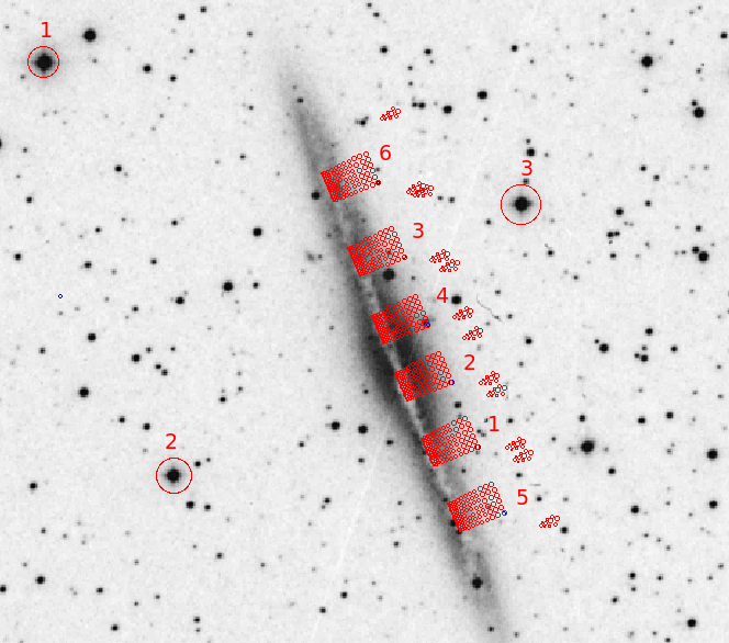
A finding chart from proposal 2014B-0456. I’ve labeled my six GradPak pointings for easy identification. The barely visible blue circles are the circles I used in step 3 above to find the location of the reference fiber (here #105). The three check stars I used are also clearly marked.

Standard Stars

Unless you really know for sure that you don’t need standard stars you should probably take some standard star observations each night. Your data reduction will be much easier if you choose standard stars that are in the IRAF database. This gives you two catalogs to choose from, the IIDS Catalog, or Massey’s Spectrophotometric Standards. Both are fine and there’s not a reason to favor one over the other.

You’ll want a few O or B stars for good flux calibration (because they don’t have many spectral lines). The more you have the better your calibration will be, but the less time you’ll spend getting data photons; the classic Astronomy tradeoff. Brighter is better because the exposures take less time, but you’ll probably be mostly limited by what stars are visible during your run. If at all possible find some stars that are visible across most of the night (at different airmasses) so you can try to get night-by-night extinction curves. On my most recent proposal this was impossible, but maybe you’ll get lucky.

If using a star from one of the catalogs mentioned the OA’s will have the coordinates already. Still, I usually put the stars in my cache just for completeness.

Airmass Charts

Airmass charts are crucial to planning out your nightly strategy; you’ll want to observe each object when it’s at the lowest possible airmass (or at least below 1.5). To generate these charts use mtools.airchart. The input file has the same format as the cache (and could even be your cache file, although that will probably clutter up the chart). You will also need to set the date of the observation, but the default latitude and longitude are already set for KPNO. Nice!

Below is an example airchart for 2014B-0456. Notice that I really needed to jump on my two standard stars at the start of the night before moving to my galaxy target. This is the kind of planning that only a good airmass chart can provide.

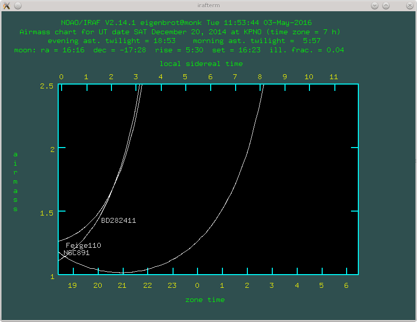
Airmass chart for December 20th, 2014. Based on this chart I spent from 19:00 to 20:00 observing my two standard stars (BD282411 and Feige 110) before they got too low on the horizon. Fortunately right around this time the galaxy NGC 891 was hitting its minimum airmass, which made for some sweet observations. It would not have been worth observing NGC 891 past about 1:30, but my program was over by 0:00 so this wasn’t a problem.

Exposure Times

Hopefully you figured this out when you wrote your proposal, but if you’re like many WIYN astronomers you probably did a lot of handwaving. Now is the time to stop waving your hands and crunch some numbers. Someday someone will write a good recipe for computing accurate exposure times on the Bench Spectrograph, but until then you’ll have to figure it out yourself. Steve Crawford’s bench simulator is a good starting point. It is out of date regarding detectors, but the grating equation never goes out of style.

Of course, you’ll want to break up your exposure times into the smallest chunks possible where you are still in the sky-limited noise regime. For a setup with 2.1 AA per pixel this was around 30 min per exposure.

Ability to Quick Reduce Data

Finally, make sure you have read (and maybe even understand) the basic flow of the Data Reduction section. At the very least you should be able to do a quick reduction of the previous night’s data before starting a new night. This way you can identify any problems like bad pointings, short exposure times, etc. while you still have a chance to fix them. It is often enough just to get through the dohydra step; flux calibration can wait.

Calibrations

Calibration frames are almost more important than the actual data; without them you entire run will be worthless. At the very least you need:

Darks: 10 darks per scientific exposure time per night is a good number. It’s OK if you can’t them every single night, but you should try to. Because the exposure times are long, it’s common to run darks during the day while you’re sleeping (set it up at the end of the night).

Zeros: Get a ton of these. Waiting for twilight? Grab some zeros! Showed up before the OA? Grab some zeros! Get lots and lots of zeros.

Flats

Getting proper flats with GradPak is different than other IFUs because the multi-pitch nature of GradPak poses some unique light-collection challenges. You may find that your spectrograph setup puts you in a position where you can’t get enough signal in the smaller fibers without saturating the large fibers:

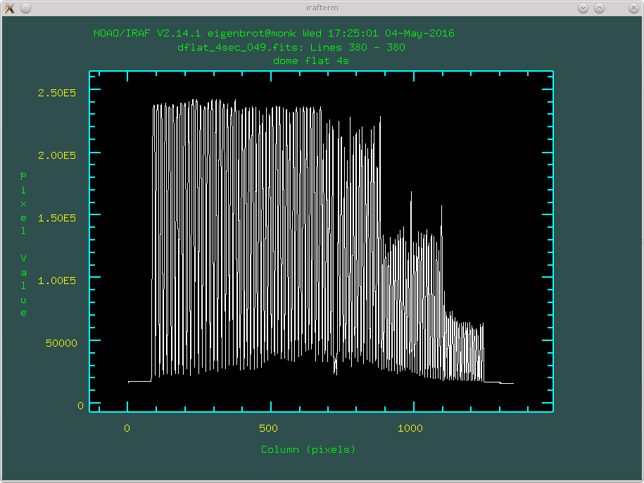
This flat has good signal in the smallest fiber (right side), but all of the large fibers are totally saturated. Not good.

If this is the case then you’ll need to take multiple flat exposures to get all fiber sizes with good signal. Deciding on what exposure times can be a little tricky but as a generaly rule you want to always look at the brightest part of the spectrum in the large fibers and the dimmest part of the spectrum in the small fibers. To say it a different way, set your short exposure time flats so that the large fibers are at the upper end of the linear regime in the brightest part of the spectrum. Similarly, set your long exposure time flats so that you get a good number of counts in the dimmest part of the spectrum with the smallest fibers.

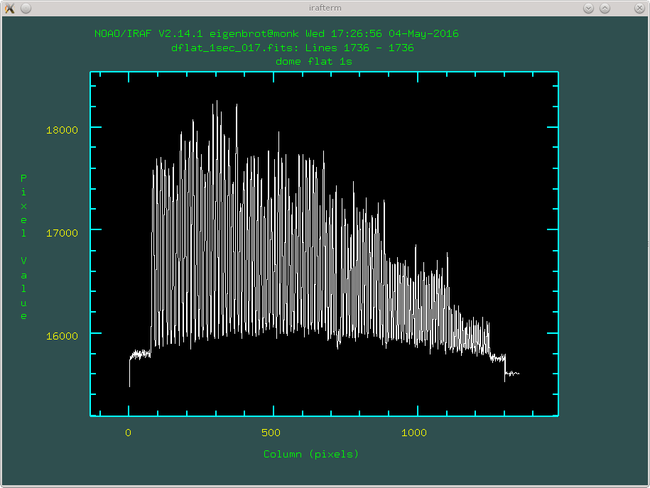
This flat has good signal in the large fibers and does not saturate where the last image did (above), but there is not enough signal in the small fibers.

It is important to note that the non-linear regime is not the same as saturating the detector; you encounter non-linearity before you saturate. This threshold varies with gain and binning, but an easy way to check is divide two flats with different exposure times. The resulting image should be constant everywhere with the value of the ratio of the exposures times. In places where there is structure you are in the non-linear regime.

In my limited experience it seems like the 2” and 3” fibers behave as the “small” fibers and the 4”, 5”, and 6” fibers are the “large” fibers.

Having said all this, make sure you actually need multiple exposure times before you go through the trouble. You might get lucky with your setup and be able to get good signal in all fibers with a single exposure time. If so, that’s awesome.

Get a statistically significant number of flats for each exposure time you need. That means at least 10.

Standard Stars

Taking standar star observations is a relatively straight forward task; simply park the star on one the fibers and expose until you get good signal. I am often surprised how long it takes to get the proper number of photons, but a minute or two is pretty typical. In a perfect world you would get light down every single fiber so you could later do a fiber-by-fiber flux calibration, but in practice you’ll probably have to settle with getting a few fibers each night.

BUT THERE IS A PROBLEM. The smallest GradPak fibers are really small. So small, in fact, that they get affected by differential atmospheric refraction (DAR). DAR causes light of different wavelengths to have slightly different focus positions at the telescope focal plane. For older Paks this wasn’t a problem because the fibers were so big that all the light from each on-sky position fell within the same fiber. Unfortunately, the 2” and 3” fibers are small enough (~200 and 300 microns, respectively. AKA, pretty damn small) that DAR causes some light to be lost off the edge of the fiber. Cruicially there is a spectrum to this lost light (that’s the very nature of DAR). In other words, you might capture all of the light redward of 5000 AA, but start loosing light off the side of the fiber at bluer wavelengths.

For observations of extended objects this isn’t that much of an issue. DAR just acts as (small) smearing kernel between you and the object. The light that is lost from one position on the sky is replaced by light added from the position right next to it.

The problem is that point sources get pretty messed up by DAR. The (wavelength dependent) light they loose does not get replaced and the end result is an artifical “DAR” spectrum imposed on top of the actual spectrum.

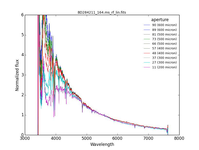
A standard star observed through multiple fiber sizes. For this observation GradPak was dragged across the standard star to sample all 5 fiber sizes. The effects of DAR are clearly visible as the supression of the blue end of the spectrum in the 3” and 2” fibers (and a little bit in the 4” fibers).

Yikes, imagine if you used the 2” fiber above to do flux calibration. Your data below 5000 AA would be completely wrong. Again, and this is very important, DAR only affects point source observations, so it is not OK to compute a “correction” from the above plot to apply to your small fibers.

So what can you do? This answer will vary based on exactly what you need standard stars for, but I can tell you what I did. Every night I took standard star observations in 3-4 6” fibers, changing the specific fibers each night. In this way I built up a collection of standard star observations for all of the fibers I know for a fact do not suffer from DAR. I then crossed my fingers and applied the resulting flux calibrations to all the rest of the fibers in the array. This is not so crazy: a good flat field calibration will remove the relative spectral differences between the fibers, then a single fiber (or group of fibers) can provide the absolute spectral calibration for the entire IFU.

In fact, we can test how legit this is. The figure below compares the absolute flux calibration across all fiber sizes. The data are taken from a single galaxy frame that has gone through all reduction steps, including flux calibration (but not sky subtraction). Each line represents the average of all 4 sky fibers for a single fiber size and all lines have been divided by the mean of all sky fibers. From this we can see that the sky spectrum in all fiber sizes is the same to within 5% for wavelengths > 4000 AA. Right around 4000 AA the 2” and 3” fibers deviate from the rest of the fibers by 10-20%, but this is just at the limit of our “good” data range (the signal drops precipitously at this point). All in all not too bad.

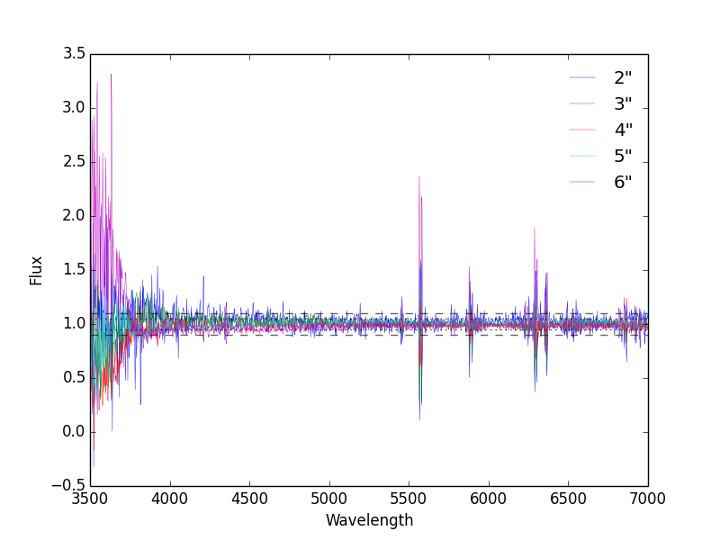
A test of the absolute flux calibration across all fiber sizes when using standard star data from only 6” fibers. The data are taken from a single galaxy exposure that has been reduced through flux calibration, but skipping sky subtraction. Each line represents the average of all 4 sky fibers for a given fiber size and all lines are normalized by the mean of all sky fibers. The dotted and dashed lines show deviations at the 5% and 10% level, respectively. All fiber sizes show an absolute flux calibration consistent within 5% for wavelengths > 4000 AA. At 4000 AA the 2” and 3” fibers deviate by up to 20%.

It’s important to note that for my actual observations I did not drag the star across the IFU (as is common for many other IFUs). For each standard star frame I placed the star in the center of a 6” and left it there the whole time. If the star is near the edge of a large fiber DAR can still caused some of the light to be lost.

Finally, I should note that it should be possible to beat the effects of DAR with some clever maneuvering. DAR disperses the light along a line normal to the horizon, i.e., azimuth. It should therefore be possible to drag the star exactly along the azimuth axis so that any light lost at time t is regained at t + epsilon. As long as the star starts and ends well off the IFU all the light should be captured by all the fibers. I spent a twilight trying this during my run and was uncessesful, which is not to say the method cannot work. If you’re feeling adventerous, go for it.